Survival analysis Kaplan-Meier using SPSS Statistics

Introduction

The Kaplan-Meier method (Kaplan & Meier, 1958), also known as the "product-limit method", is a nonparametric method used to estimate the probability of survival past given time points (i.e., it calculates a survival distribution). Furthermore, the survival distributions of two or more groups of a between-subjects factor can be compared for equality.

For example, in a study on the effect of drug dose on cancer survival in rats, you could use the Kaplan-Meier method to understand the survival distribution (based on time until death) for rats receiving one of four different drug doses: "40 mg/m²/d", "80 mg/m²/d", "120 mg/m²/d" and "160 mg/m²/d" (i.e., the survival time variable would be "time to death" and the between-subjects factor would be "drug dose"). You could then compare the survival distributions (experiences) between the four doses to determine if they are equal. If they were not equal, you could further determine where any differences between the groups of the between-subjects factor lie (e.g., whether death rates were higher in rats given the lowest drug dose – "40 mg/m²/d" of the drug – compared to rats given the highest drug dose: "160 mg/m²/d"). Alternately, you could use the Kaplan-Meier method to determine whether the (distribution of) time to failure of a knee replacement differs based on exercise impact amongst young patients (i.e., the survival time would be "time to knee replacement failure" and the between-subjects factor would be "exercise impact", which has three groups: "sedentary", "low impact" and "high impact"). You could then compare the survival distributions (experiences) between the three levels of exercise impact to determine if they are equal, and if not, where any differences lie (e.g., whether time to knee replacement failure was lower in the "sedentary" exercise group compared to the "high impact" exercise group).

This "quick start" guide shows you how to carry out a Kaplan-Meier analysis using SPSS Statistics, as well as interpret and report the results from this analysis. However, before we introduce you to the SPSS Statistics procedure to perform a Kaplan-Meier analysis, you need to understand the different assumptions that you must meet in order to use the Kaplan-Meier method. We discuss these assumptions next.

SPSS Statisticstop ^

Assumptions

The Kaplan-Meier method has six assumptions that must be met. If these assumptions are not met, you cannot use the Kaplan-Meier method, but may be able to use another type of survival analysis instead. Therefore, before you can use the Kaplan-Meier method using SPSS Statistics, you need to check that you have met the following six assumptions:

• Assumption #1: The event status should consist of two mutually exclusive and collectively exhaustive states: "censored" or "event" (where the "event" can also be referred to as "failure"). The event status is mutually exclusive because the outcome for a case can either be censored or the event has occurred. It cannot be both. For example, imagine that we were interested in the survival times of people suffering from skin cancer, where the event is "death". If the length of the experiment was 5 years, at the end of the 5-year period, all participants would either be "censored" or "dead". Therefore, the two states should not only be mutually exclusive, but also collectively exhaustive (i.e., at least one of these states – censored or event – must occur).
• Assumption #2: The time to an event or censorship (known as the "survival time") should be clearly defined and precisely measured. The Kaplan-Meier method, unlike some other approaches to survival analysis (e.g., the actuarial approach), requires the survival time to be recorded precisely (i.e., exactly when the event or censorship occurred) rather than simply recording whether the event occurred within some predefined interval (e.g., only recording when a death or censorship occurred sometime within a 1, 2, 3, 4 and 5 year follow-up). In addition, the survival time should be clearly defined, whether this is measured in days, weeks, months, years, or some other time-based measurement.
• Assumption 3: Where possible, left-censoring should be minimized or avoided. Left-censoring occurs when the starting point of an experiment is not easily identifiable. Again, imagine that we were interested in the survival times of people suffering from skin cancer. The "ideal" starting point would be to measure the survival time from the very moment that the participant developed skin cancer. However, it is more likely that the first time the participant knew they had cancer was the moment it was diagnosed, such that the "diagnosis" acts as the starting point for the experiment. Even if we isolated our sample to a "Stage 1" cancer diagnosis, there will still be differences between participants. For example, some participants may have had a suspicious mole that they did not get checked for some time, whilst other participants may have regular check-ups such that a diagnosis was made much earlier. Therefore, the time between the participant developing skin cancer and the diagnosis is "unknown" and is "not included" in the Kaplan-Meier analysis. The result is that this data – known as left-censored data – does not reflect the observed survival time. Instead, the survival time recorded will be less than (or equal to) the observed survival time. As such, the goal is to avoid left-censoring as much as possible.
• Assumption 4: There should be independence of censoring and the event. This means that the reason why cases are censored does not relate to the event. For the assumption of independent censoring to be met, we need to be confident that when we record that a participant is "censored", this is not because they were at greater risk of the event occurring (i.e., "death" being the "event" in this case). Instead, there may be many other reasons why a participant is "legitimately censored", including: (a) natural dropout or withdrawal (e.g., perhaps because the participant does not want to take part in the experiment any more or moves away from the area); and (b) the event not occurring by the end of the experiment (e.g., if the follow-up period for the experiment is 5 years, any participant still alive at this point will be recorded as "censored"). Independent censoring is important because the Kaplan-Meier method is based on observed data (i.e., observed events) and assumes that censored data behaves in the same way as uncensored data (after the censoring). However, if the censored data does relate to the event (e.g., a participant that was recorded as being censored died due to the cancer or perhaps even something related to the cancer), this introduces serious bias to the results (e.g., over-estimating 5-year survival rates from skin cancer amongst participants).
• Assumption 5: There should be no secular trends (also known as secular changes). A characteristic of many studies that involve survival analysis is that: (a) there is often a long time period between the start and end of the experiment; and (b) not all cases (e.g., participants) tend to start the experiment at the same time. For example, the starting point in our hypothetical experiment was when participants were "diagnosed" with skin cancer. However, imagine that we wanted a sample of 500 participants in our experiment. It may take a number of months to recruit all of these participants, each of whom would have different starting points (i.e., the dates when they were diagnosed), but we would "pool" the starting and subsequent times (e.g., everybody's first diagnosis would be time point 0). However, if over this period of time, factors have changed that affect the likelihood of the event, this may introduce bias. For example, death rates for skin cancer may have gone down following the introduction of new drugs, improving survival rates amongst participants joining the experiment later on. Alternately, the introduction of a national skin-screening programme may have led to faster diagnoses, increasing the perception of worse survival rates amongst participants who started the study before the programme was introduced (i.e., by reducing left-censoring). These factors (e.g., new drugs or better screening) are examples of secular trends that can bias the results.
• Assumption 6: There should be a similar amount and pattern of censorship per group. One of the assumptions of the Kaplan-Meier method and the statistical tests for differences between group survival distributions (e.g., the log rank test, which we discuss later in the guide) is that censoring is similar in all groups tested. This includes a similar "amount" of censorship per group and similar "patterns" of censorship per group. Failure to meet the assumption can lead to false conclusions being drawn about differences in group survival distributions (i.e., rejection or not of the null hypothesis), based on these statistical tests "confusing" differences in censoring patterns with actual group differences in survival distributions (Bland & Altman, 2004; Hosmer et al., 2008; Norušis, 2012).
  
  To detect censoring, you can use SPSS Statistics: (a) to calculate the percentage of censored cases (e.g., participants) per intervention group to determine whether there is a similar "amount" of censorship per group; and (b) to produce a scatterplot illustrating the "pattern" of censoring. We show you how to generate a table of the percentage of censored cases using SPSS Statistics, as well as how to generate the scatterplot of censored cases to determine the "pattern" of censorship per group in our enhanced Kaplan-Meier guide. You can access this enhanced guide by subscribing to the site here.

If your study design does not meet these six assumptions, you might not be able to use the Kaplan-Meier method. If you would like to know more about the characteristics of the Kaplan-Meier method, including the null and alternative hypotheses it is testing, see our enhanced Kaplan-Meier guide. In the section, Test Procedure in SPSS Statistics, we show you how to analyse your data using the Kaplan-Meier method in SPSS Statistics. First, we introduce you to the example we use in this guide.

TAKE THE TOUR

PLANS & PRICING

SPSS Statisticstop ^

Example

A researcher wanted to determine the relative effectiveness of three types of intervention designed to help long-term smokers quit: a "hypnotherapy programme", wearing "nicotine patches" and the use of "e-cigarettes" (electronic cigarettes). More specifically, the researcher wanted to determine if and when smokers that had quit smoking after undertaking one of these three interventions started smoking again. Participants were observed for 2 years (104 weeks) after the interventions had taken place. A successful result would be where smokers did not start smoking again. Also, the longer the length of time it took before participants started smoking again, the more effective the intervention. For example, if participants that used the e-cigarettes largely started to smoke again towards the end of the second year, but those participants using nicotine patches started smoking again in the middle of the first year, the researcher could consider the e-cigarette intervention to be more effective. Therefore, the Kaplan-Meier method was used to help achieve two goals:

• First, to determine whether there were statistically significant differences between the survival distributions of the three interventions: In our example, we have three survival distributions reflecting the three groups of our between-subjects factor intervention (i.e., the three groups are the three interventions: the "hypnotherapy programme", "nicotine patch" and use of "e-cigarette" groups). The survival distributions illustrate how survival time, time, (expressed as the cumulative survival probability) differed between the three interventions over time. These three survival distributions (derived by the Kaplan-Meier method) can be tested to determine whether there are any statistically significant differences between them.
• Second, if there were statistically significant differences between the survival distributions, you can then determine which specific interventions differed from each other: That is, having established that these survival distributions are different between the three groups, you will want to establish which specific groups were different (i.e., which survival distributions of the groups of the between-subjects factor differed from each other). For example, we may want to know whether there was a difference in the survival distribution of participants that underwent the hypnotherapy programme compared to those using nicotine patches; or whether there was a difference between those using the nicotine patches versus the e-cigarettes. If we make all possible comparisons between groups – which is what SPSS Statistics does – these comparisons are known as "all pairwise comparisons". You will only need to run pairwise comparisons if you have three or more groups.

Therefore, the researcher recruited a sample of 150 participants to the study. These 150 participants were randomly divided into three independent groups of 50 participants, with 50 participants undergoing the hypnotherapy programme, another 50 participants using the nicotine patches and the final 50 using the e-cigarettes.

At the end of the three interventions (during the 2-year follow-up period), the researcher recorded whether a participant started smoking again, which was defined as the "event". If the participant did not start smoking again or dropped out of the study, the researcher recorded this participant as being "censored". These two options – an "event" or being "censored" – reflect the two categories of the event status variable, which we have simply called status. The time until a participant either reaches the "event" or is "censored" is called the survival time and is measured in the variable, time. This time could be from 0 weeks (i.e., immediately after a participant finishes the intervention) through to 104 weeks (i.e., 2 years after the intervention when the researcher decided to determine the relative success of the three interventions).

SPSS Statisticstop ^

Setup in SPSS Statistics

For a Kaplan-Meier survival analysis, you will have at least four variables. In this example, these are:

• 1) The case identifier, id, which simply lets SPSS Statistics distinguish between each case (i.e., participant) during the Kaplan-Meier procedure.
• 2) The survival time variable, time, which is the time until an event occurs or when the data becomes censored. In this example, survival time is measured in weeks from 0 weeks to a cut-off of 104 weeks (i.e., 2 years).
• 3) The event status variable, status, which has two groups: "censored" (i.e., where participants dropped out of the study or the event did not occur by the end of the study) and "event" (i.e., where the event occurred, which in this study is when participants started to smoke again).
• 4) The between-subjects factor, intervention, which consists of the groups that you are comparing. In this example, the between-subjects factor reflects the intervention that is given to participants, which consists of three groups: the "hypnotherapy programme", "nicotine patch" and "e-cigarette" groups.

If you are unsure how to correctly enter these variables into the Variable View and Data View of SPSS Statistics so that you can carry out your analysis, we show you how to do this in our enhanced Kaplan-Meier guide. You can learn about our enhanced data setup content in general here or subscribe to the site here to access our enhanced Kaplan-Meier guide.

SPSS Statisticstop ^

Test Procedure in SPSS Statistics

The 13 steps below show you how to analyse your data using the Kaplan-Meier method in SPSS Statistics to determine whether there are statistically significant differences in the survival distributions between the groups of your between-subjects factor using the log rank test, Breslow test and Tarone-Ware test. At the end of these 13 steps, we show you how to interpret the results from this test.

• Click Analyze > Survival > Kaplan-Meier... on the main menu:
  

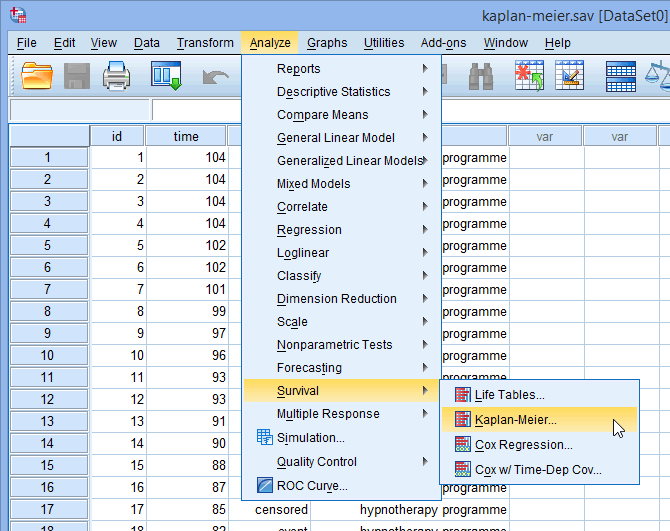  Published with written permission from SPSS Statistics, IBM Corporation.
  You will be presented with the Kaplan-Meier dialogue box, as shown below:
  

  Published with written permission from SPSS Statistics, IBM Corporation.
• Transfer the survival time variable, time, into the Time: box, the between-subjects factor variable, intervention, into the Factor: box, and the case identifier, id, into the Label Cases by: box, by selecting each relevant variable (by clicking on it) and then clicking the relevant  button. You will end up with the following screen:
  

  Published with written permission from SPSS Statistics, IBM Corporation.
• Transfer the event status variable, status, into the Status: box, by selecting it (by clicking on it) and then clicking the relevant  button. You will end up with the following screen:
  

  Published with written permission from SPSS Statistics, IBM Corporation.
• Click the  button. You will be presented with the Kaplan-Meier: Define Event For Status dialogue box, as shown below:
  Note: If the  button is not active (i.e., it looks faded like this, ), make sure that the event status variable, status, is highlighted in yellow (as above) by clicking on it. This will activate the  button.
  

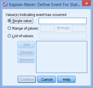  Published with written permission from SPSS Statistics, IBM Corporation.
• Enter "1" into the Single value: box, as shown below:
  

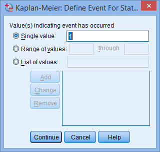  Published with written permission from SPSS Statistics, IBM Corporation.
  Explanation: We entered "1" because this reflects the code assigned to the event occurring in our example (i.e., a participant starting to smoke again). This should mirror the way you set up your data in the Variable View of SPSS Statistics. In our example, "0" meant that the data was "censored" and "1" that the "event" occurred. If you are unsure how to set up this coding in the Value Labels dialogue box in SPSS Statistics, we should you how in our enhanced Kaplan-Meier guide, which you can access by subscribing to the site here.
• Click the  button and you will be returned to the Kaplan-Meier dialogue box, but now with a completed Status: box, as shown below:
  

  Published with written permission from SPSS Statistics, IBM Corporation.
• Click the  button and you will be presented with the Kaplan-Meier: Options dialogue box, as shown below:
  

  Published with written permission from SPSS Statistics, IBM Corporation.
• Leave the Survival table(s) and Mean and median survival checkboxes ticked in the –Statistics– area and select the Survivalcheckbox in the –Plots– area. You should end up with the following screen:
  

  Published with written permission from SPSS Statistics, IBM Corporation.
• Click the  button and you will be returned to the Kaplan-Meier dialogue box.
• Click the  button and you will be presented with the Kaplan-Meier: Compare Factor Levels dialogue box, as shown below:
  

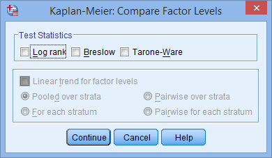  Published with written permission from SPSS Statistics, IBM Corporation.
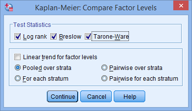
• Click the Log rank, Breslow and Tarone-Ware checkboxes in the –Test Statistics– area and leave the Pooled over strataoption selected. You should end up with the following screen:
  

  Published with written permission from SPSS Statistics, IBM Corporation.
• Click the  button and you will be returned to the Kaplan-Meier dialogue box.
• Click the  button to generate the output for the Kaplan-Meier test.

Now that you have run the Kaplan-Meier procedure, we show you how to interpret and report your results.

Join the 10,000s of students, academics and professionals who rely on Laerd Statistics.TAKE THE TOUR PLANS & PRICING

SPSS Statisticstop ^

Output from using the Kaplan-Meier method in SPSS Statistics

SPSS Statistics generates quite a lot of output for the Kaplan-Meier method: the Survival Functions and Censoring plots, and a number of tables: the Means and Medians for Survival Time, Case Processing Summary and Overall Comparisons tables. If you have statistically significant differences between the survival functions, you will also need to interpret the Pairwise Comparisons table, allowing you to determine where the differences between your groups lie. In the sections below, we focus on the Overall Comparisons table, as well as touching on the Survival Functions plot.

Note: If you are unsure how to interpret and report the descriptive statistics from the Mean and Medians for Survival Time table, or the the percentages from the Case Processing Summary table, which is part of the assumption testing we discussed in the Assumptions section earlier, we show you how to do this in our enhanced Kaplan-Meier guide. If you find that you have statistically significant differences between your survival distributions, we also explain how to interpret and report the Pairwise Comparisons table. You will also need to run additional procedures in SPSS Statistics to carry out these pairwise comparisons because the 13 steps in the Test Procedure in SPSS Statistics section above do not include the procedure for pairwise comparisons.

SPSS Statisticstop ^

Survival functions

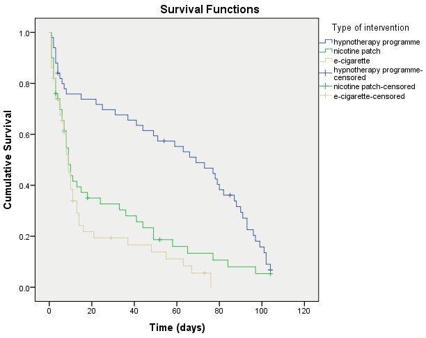
The first and best place to start understanding and interpreting your results is usually with the plot of the cumulative survival functions for the different groups of the between-subjects factor (i.e., the three groups of intervention: the "hypnotherapy programme", "nicotine patch" and use of "e-cigarette" groups). This is a plot of the cumulative survival proportion against time for each intervention group and is labelled the Survival Functions plot in SPSS Statistics. This plot is shown below:

Published with written permission from SPSS Statistics, IBM Corporation.

The plot above will help you to understand how the survival distributions compare between groups. A useful function of the plot is to illustrate whether the survival curves cross each other (i.e., whether there is an "interaction" between survival distributions). This has implications on the power of the statistical tests to detect differences between the survival distributions. In addition, you should decide whether the survival curves are similarly shaped, even if they are above or below one another. This has implications for the choice of statistical test that is used to analyse the results from the Kaplan-Meier method (i.e., whether you use the log rank test, Breslow test or Tarone-Ware test, as discussed later).

The "event" you are interested in is usually considered to be delirious (e.g., failure or death). Therefore, it is not something you want to occur. All other things being equal (e.g., censoring of cases), the more events that occur, the lower the cumulative survival proportion and the lower (i.e., on the y-axis) the survival curve on the graph. As such, a group survival curve that appears "above" another group's survival curve is usually considered to be demonstrating a beneficial/advantageous effect.

We can see from our plot that the cumulative survival proportion appears to be much higher in the hypnotherapy group compared to the nicotine patch and e-cigarette groups, which do not appear to differ considerably (although the nicotine patch intervention appears to have a small advantage on survival; that is, fewer participants resuming smoking). It would appear that the hypnotherapy programme significantly prolongs the time until participants resume smoking (i.e., the event) compared to the other interventions. However, if we inspect the curves' last cumulative survival proportion, we can see that the proportion of participants that had not resumed smoking by the end of the study does not appear that different between the intervention groups (at approximately 10%). We will look into determining if these survival curves are statistically significantly different later.

Note: Having inspected the cumulative survival plot in the previous section, it is a good idea to look at the descriptive elements from your results using the Means and Medians for Survival Time table. This will help to clarify the various survival times for your groups. To do this, you need to interpret the median values and their 95% confidence intervals. You can also plot the median survival times of the groups on top of the survival plot illustrated above. In our enhanced Kaplan-Meier guide, we explain how to interpret and report the SPSS Statistics output from the Means and Medians for Survival Time table.

SPSS Statisticstop ^

Choosing between statistical tests: The log rank test, Breslow test and Tarone-Ware test

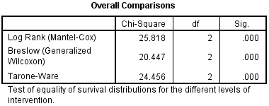
There are three statistical tests that can be selected in SPSS Statistics that test whether the survival functions are equal. These are the log rank test (Mantel, 1966), Breslow test (Breslow, 1970; Gehan, 1965) and the Tarone-Ware test (Tarone & Ware, 1977), all of which we selected to be produced in the Test Procedure in SPSS Statistics section above. These three tests are presented in the Overall Comparisons table, as shown below:

Published with written permission from SPSS Statistics, IBM Corporation.

All three tests compare a weighted difference between the observed number of events (i.e., the resumption of smoking) and the number of expected events at every time point, but differ in how they calculate the weight. We discuss the differences between these three statistical tests and which test to choose in our enhanced Kaplan-Meier guide.

It is fairly common to find that all three tests will lead you to the same conclusion (i.e., they will all reject the null hypothesis or they all won't), but which test you choose should depend on how you expect the survival distributions to differ so as to make best use of the different weightings each test assigns to the time points (i.e., increase statistical power). Unfortunately, you cannot rely on there being one best test – it will depend on your data. If you choose the approach of picking a particular test, you will need to do this before analysing your data. You shouldn't run all of them and then simply pick the one that happens to have the "best" p-value for your study (Hosmer et al., 2008; Kleinbaum & Klein, 2012).

In our example, the log rank test is the most appropriate, so we discuss the results from this test in the next section.

SPSS Statisticstop ^

Comparison of interventions

To use the log rank test, you need to interpret the "Log Rank (Mantel-Cox)" row in the Overall Comparisons table, as highlighted below:

Published with written permission from SPSS Statistics, IBM Corporation.

The log rank test is testing the null hypothesis that there is no difference in the overall survival distributions between the groups (e.g., intervention groups) in the population. To test this null hypothesis, the log rank test calculates a χ²-statistic (the "Chi-Square" column), which is compared to a χ²-distribution with two degrees of freedom (the "df" column). In order to determine whether the survival distributions are statistically significantly different, you need to consult the "Sig." column which contains the p-value for this test. You can see that the significance value of this test is .000. This does not mean that p = .000, but that p < .0005. If you want to know the actual p-value, you can double-click the table and hover your mouse over the relevant p-value, as highlighted below:

Published with written permission from SPSS Statistics, IBM Corporation.

You can now see that the p-value is actually .000002 (i.e., p = .000002). The reason for it initially appearing that p = .000 is due to the result only being reported in the table to 3 decimal places. However, it is rare that you would quote such a small p-value, so you might simple state that p < .0005.

If p < .05, you have a statistically significant result and can conclude that the survival distributions of the different types of intervention are not equal in the population (i.e., they are not all the same). On the other hand, if p > .05, you do not have a statistically significant result and cannot conclude that the survival distributions are different in the population (i.e., they are all the same/equal). In this example, since p = .000002, we have a statistically significant result. That is, the survival distributions are different in the population.